Postdoc, University of Twente
Mathematics Teacher, Carmel College Salland
A perfect strategy for roulette?
This case study uses SCOOP to model a strategy for the roulette casino game. Combining forces with CADP and MRMC, we compute the probability of going home with a profit.The game
The game of roulette goes as follows: the dealer spins a little ball, which lands on a number between 0 and 36 according to a uniform distribution. Hence, the probability of each outcome is 1/37. The player can bet on several items, two of which are the guess that the outcome is either even or odd. He wins if the actual outcome corresponds to his guess (except for the outcome 0, in which case nobody wins).We explore a strategy that seems to maximise our probability of winning. Basically, we just always guess on even and double the stakes each time we loose. Initially we bet 1 euro. If we win, we go home with a profit. If we loose, we bet 2 euros. Again, if we win we go home, otherwise we bet 4 euros. It is easy to see that, no matter how many times we loose, at some point we will win and then receive precisely the amount of money we lost so far increased by 1 euro. Hence, we will always go home 1 euro richer.
Unfortunately, in practice this strategy will not always work. After all, the amount of money we bet increases exponentially with the number of losses, so we will quickly be out of money and therefore not able to continu the strategy. Additionally, several casino's have put a limit on the amount of money that can be bet in one round.
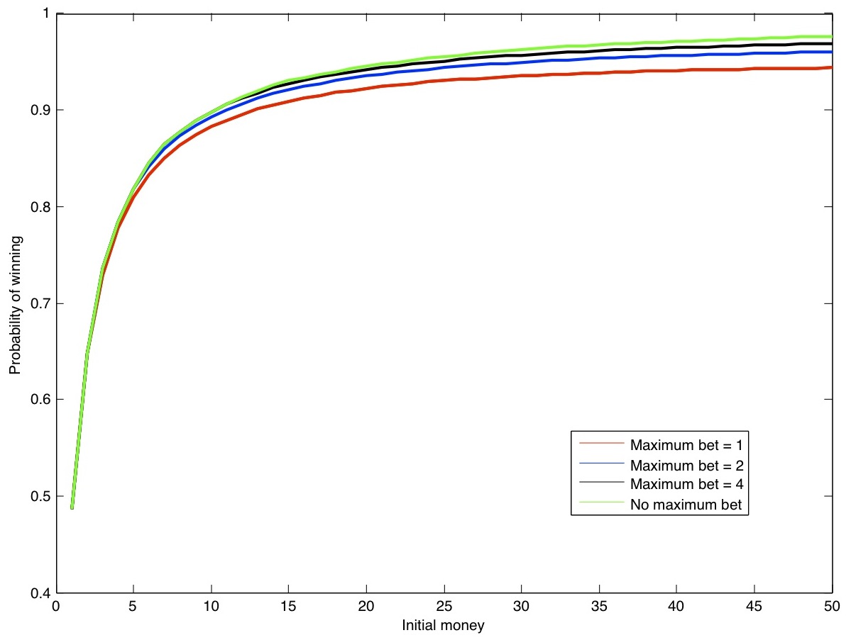
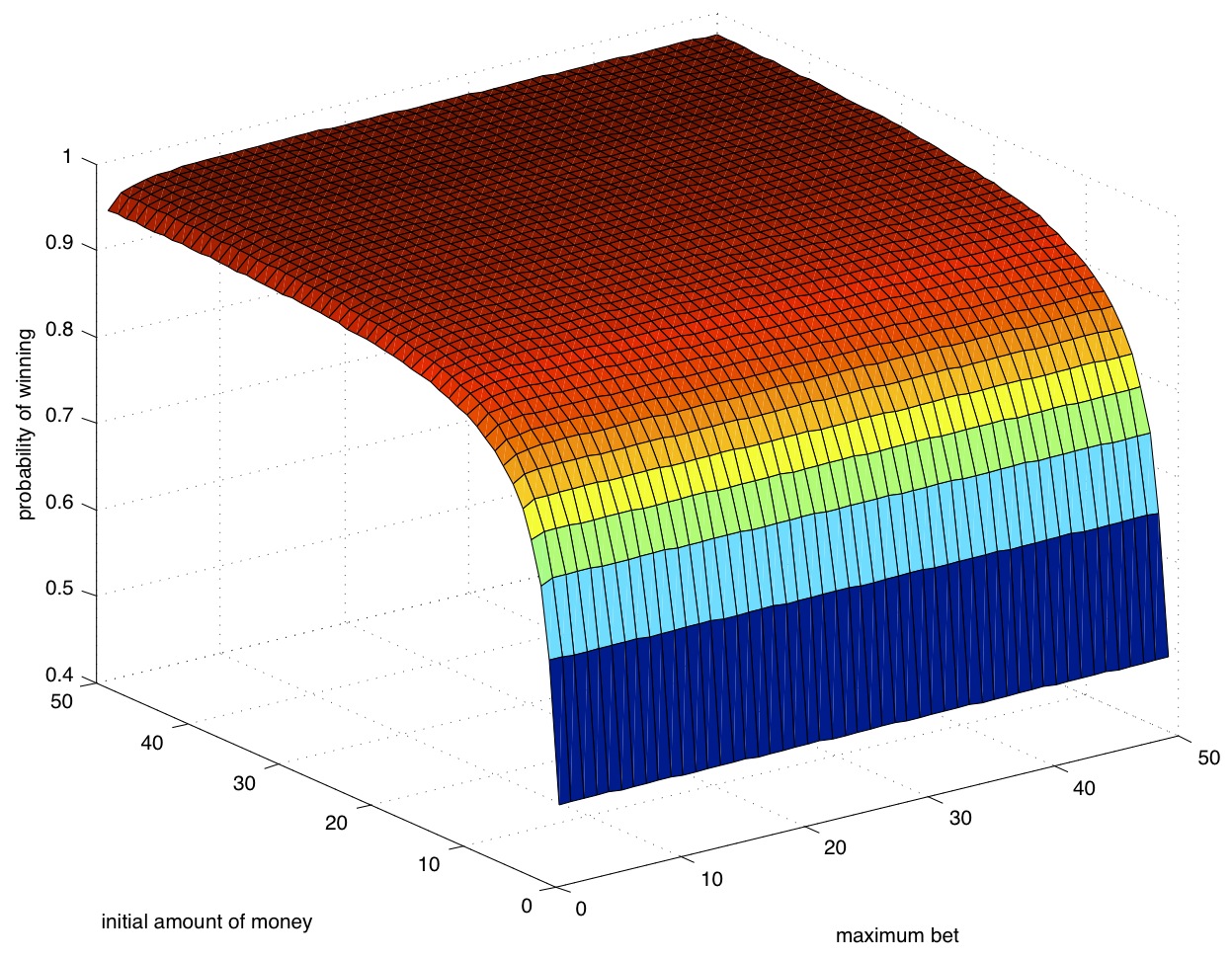
Based on the observations above, we investigate the winning probabilities of this strategy for different initial amount of money and different betting limits.
The SCOOP model
It is not so difficult to model this game, including the strategy, in SCOOP.For ease of modelling, we introduce four types:
type Bet = {1..2*maximumBet}
type Money = {0..initialMoney+1}
type Outcome = {0..36}
type Guess = (even, odd)
The types are based on two constants, which will be instantiated during the state space generation:
maximumBet and initialMoney. Note that the amount of money we have never
exceeds the initial amount increased by 1, since the strategy forces us to go home after reaching precisely this point.
At some point the bet may be more than the maximum bet, but this will be resolved later on.
Based on these types, we can model some processes. First, we model the player:
SmartPlayer(m:Money, nextBet:Bet) =
m = 0 | m > initialMoney => Finished[m]
++ m > 0 & m <= initialMoney => Play[m,min(m, min(nextBet, maximumBet))]
A player is characterised by the amount of money he has, and by the amount of money he will
bet in the next round. If he doesn't have any money left or made a profit, he quits.
Otherwise, he will bet again, following our strategy. Note that it is only possible
to follow the strategy if we have enough money and if the betting limit
does not prohibit us from betting the required amount. Therefore, we take a minimum
over the amount of money we have, the limit and the bet according to the strategy.
In case the game in finished, we output the result:
Finished(m:Money) =
m = 0 => broke . Finished[m]
++ m > 0 => quit(m) . Finished[m]
In case we play, we guess even, the dealer spins the ball and we obtain an outcome.
Instead of giving each outcome a probability of 1/37, we chose to give 1 and 2 both a probability of
18/37, to give 0 a probability of 1/37 and to give a probability of 0 to all other outcomes.
Clearly, this is equivalent to the actual situation, it doesn't matter which specific number we get,
only whether it is odd, even, or 0.
Play(m:Money, b:Bet) =
guess(even). deal. psum(o:Outcome,
ifthenelse(o=1, 18/37,
ifthenelse(o=2, 18/37,
ifthenelse(o=0, 1/37, 0))):
outcome(o) . (o = 0 => loose.SmartPlayer[m-b,b*2]
++ o > 0 => Decision[even,o,m,b]))
If the outcome is 0, we lost. In that case, we continu after subtracting the bet from our amount of money and doubling the bet.
Otherwise, we use the process Decision to decide on the outcome of the bet.
It checks whether the parity of the outcome corresponds to the guess. If not, we continu as above.
If so, the bet is added to our amount of money and in the bet for the next round is set to 1. (Note that winning one round does not
immediately implies that we made a profit and will quit; after all,it could be the case that our bet was lower than what is
prescribed by the strategy, due to us running out of cash or not being allowed to exceed the table limit.)
Decision(g:Guess, o:Outcome, m:Money, b:Bet) =
g = even => (mod(o,2) = 0 => win.SmartPlayer[m+b,1]
++ mod(o,2) = 1 => loose.SmartPlayer[m-b,2*b])
++ g = odd => (mod(o,2) = 1 => win.SmartPlayer[m+b,1]
++ mod(o,2) = 0 => loose.SmartPlayer[m-b,2*b])
Finally, the model has to be initiated and some actions can be hidden.
init SmartPlayer[initialMoney,1]
hide guess, deal, win, outcome, loose
The complete model is incorporated in the web-based version of SCOOP, and can
also be found here.
Analysing the model
It is easy to let SCOOP generate a state space of this model, but in the end we are interested in the probability of going home with a profit. For this, we will use the model checker MRMC. Since SCOOP only uses heurstics for reducing the model size, clearly in general it does not generate the minimal probabilistic automaton. Therefore, it turns out that we can best first minimise the state space modulo probabilistic branching bisimulation, before feeding it to MRMC. For this minimisation step, the BCG_MIN tool of the CADP toolset is perfectly applicable.The steps we take to minimise the state space are as follows:
- scoop -conf -aut -cadp -dtmc -constant-initialMoney=100 -constant-maximumBet=10 < roulette.prcrl > roulette.aut
- bcg_io -aldebaran roulette.aut -bcg roulette.bcg
- bcg_min -branching -prob roulette.bcg rouletteReduced.bcg
- bcg_io -bcg rouletteReduced.bcg -aldebaran rouletteReduced.aut
To simplify things, we created a small Java program that takes an AUT file and produces the corresponding TRA and LAB files that are asked for by MRMC. It can be downloaded here and applied as follows:
- javac -classpath . AUTtoTRA.java
- java -classpath . AUTtoTRA rouletteReduced.aut
Finally, we can apply MRMC to compute the probability of going broke. We need the following commands:
P {>= 0 } [tt U broke]
$RESULT[1]
A file that contains these (plus some additional commands to switch off debug information) can be found here.
It can be applied as follows:
- mrmc dtmc rouletteReduced.aut.tra rouletteReduced.aut.lab < roulette.mrmc
Experimenting with several instances of the model
We are interested in finding out the probability of winning for a variety of values for initialMoney and maximumBet. Therefore, we used this script to perform the above steps for all combinations (i,j) for these variables for 1 <= i,j <= 50. The script uses an additional little program to parse the output of MRMC. It can be compiled using- javac -classpath . ParseMRMC.java